tobac Feature Detection Filtering

Often, when detecting features with tobac, it is advisable to perform some amount of filtering on the data before feature detection is processed to improve the quality of the features detected. This notebook will demonstrate the affects of the various filtering algorithms built into tobac feature detection.

Imports

%matplotlib inline
import matplotlib.pyplot as plt
import numpy as np
import tobac
import xarray as xr
import scipy.ndimage
import skimage.morphology

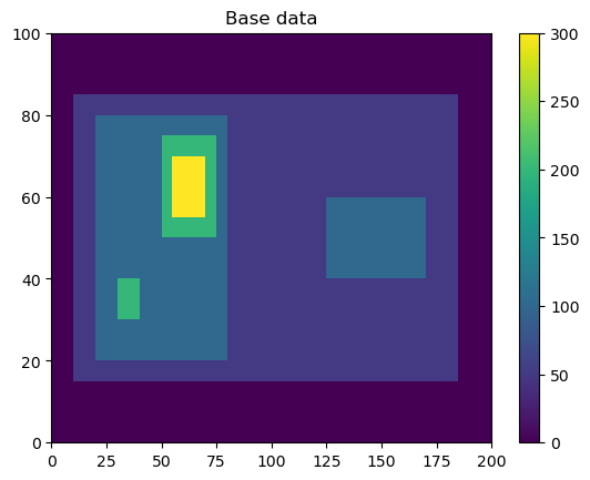
Generate Feature Data

Here, we will generate some simple feature data where the features that we want to detect are higher values than the surrounding (0).

# Dimensions here are time, y, x.
input_field_arr = np.zeros((1,100,200))
input_field_arr[0, 15:85, 10:185]=50
input_field_arr[0, 20:80, 20:80]=100
input_field_arr[0, 40:60, 125:170] = 100
input_field_arr[0, 30:40, 30:40]=200
input_field_arr[0, 50:75, 50:75]=200
input_field_arr[0, 55:70, 55:70]=300

plt.pcolormesh(input_field_arr[0])
plt.colorbar()
plt.title("Base data")
plt.show()

# We now need to generate an Iris DataCube out of this dataset to run tobac feature detection.
# One can use xarray to generate a DataArray and then convert it to Iris, as done here.
input_field_iris = xr.DataArray(input_field_arr, dims=['time', 'Y', 'X'], coords={'time': [np.datetime64('2019-01-01T00:00:00')]}).to_iris()
# Version 2.0 of tobac (currently in development) will allow the use of xarray directly with tobac.

/var/folders/40/kfr98p0j7n30fjp2n4ljjqbh0000gr/T/ipykernel_51487/1365866487.py:3: UserWarning: Converting non-nanosecond precision datetime values to nanosecond precision. This behavior can eventually be relaxed in xarray, as it is an artifact from pandas which is now beginning to support non-nanosecond precision values. This warning is caused by passing non-nanosecond np.datetime64 or np.timedelta64 values to the DataArray or Variable constructor; it can be silenced by converting the values to nanosecond precision ahead of time.
  input_field_iris = xr.DataArray(input_field_arr, dims=['time', 'Y', 'X'], coords={'time': [np.datetime64('2019-01-01T00:00:00')]}).to_iris()

---

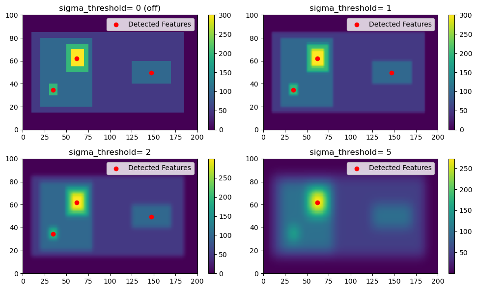
Gaussian Filtering (sigma_threshold parameter)

First, we will explore the use of Gaussian Filtering by varying the sigma_threshold parameter in tobac. Note that when we set the sigma_threshold high enough, the right feature isn’t detected because it doesn’t meet the higher 100 threshold; instead it is considered part of the larger parent feature that contains the high feature.

thresholds = [50, 100, 150, 200]
fig, axarr = plt.subplots(2,2, figsize=(10,6))
sigma_values = [0, 1, 2, 5]
for sigma_value, ax in zip(sigma_values, axarr.flatten()):
    single_threshold_features = tobac.feature_detection_multithreshold(field_in = input_field_iris, dxy = 1000, threshold=thresholds, target='maximum', sigma_threshold=sigma_value)

    # This is what tobac sees
    filtered_field = scipy.ndimage.gaussian_filter(input_field_arr[0], sigma=sigma_value)
    color_mesh = ax.pcolormesh(filtered_field)
    plt.colorbar(color_mesh, ax=ax)
    # Plot all features detected
    ax.scatter(x=single_threshold_features['hdim_2'].values, y=single_threshold_features['hdim_1'].values, color='r', label="Detected Features")
    ax.legend()
    if sigma_value == 0:
        sigma_val_str = "0 (off)"
    else:
        sigma_val_str = "{0}".format(sigma_value)
    ax.set_title("sigma_threshold= "+ sigma_val_str)
plt.tight_layout()
plt.show()

---

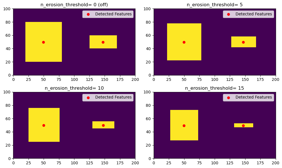
Erosion (n_erosion_threshold parameter)

Next, we will explore the use of the erosion filtering by varying the n_erosion_threshold parameter in tobac. This erosion process only occurrs after masking the values greater than the threshold, so it’s easiest to see this when detecting on a single threshold. As you can see, increasing the n_erosion_threshold parameter reduces the size of each of our features.

thresholds = [100]
fig, axarr = plt.subplots(2,2, figsize=(10,6))
erosion_values = [0, 5, 10, 15]
for erosion, ax in zip(erosion_values, axarr.flatten()):
    single_threshold_features = tobac.feature_detection_multithreshold(field_in = input_field_iris, dxy = 1000, threshold=thresholds, target='maximum', n_erosion_threshold=erosion)

    # Create our mask- this is what tobac does internally for each threshold.
    tobac_mask = 1*(input_field_arr[0] >= thresholds[0])

    if erosion > 0:
        # This is the parameter for erosion that gets passed to the scikit-image library.
        footprint = np.ones((erosion, erosion))
        # This is what tobac sees after erosion.
        filtered_mask = skimage.morphology.binary_erosion(tobac_mask, footprint).astype(np.int64)
    else:
        filtered_mask = tobac_mask

    color_mesh = ax.pcolormesh(filtered_mask)
    # Plot all features detected
    ax.scatter(x=single_threshold_features['hdim_2'].values, y=single_threshold_features['hdim_1'].values, color='r', label="Detected Features")
    ax.legend()
    if erosion == 0:
        sigma_val_str = "0 (off)"
    else:
        sigma_val_str = "{0}".format(erosion)
    ax.set_title("n_erosion_threshold= "+ sigma_val_str)
plt.tight_layout()
plt.show()