Methods and Parameters for Feature Detection: Part 1
In this notebook, we will take a detailed look at tobac’s feature detection and examine some of its parameters. We concentrate on:
Minima/Maxima and Multiple Thresholds for Feature Identification
[1]:
import matplotlib.pyplot as plt
import numpy as np
import xarray as xr

%matplotlib inline

import seaborn as sns

sns.set_context("talk")

import warnings

warnings.filterwarnings("ignore")
[2]:
import tobac
import tobac.testing
Minima/Maxima and Multiple Thresholds for Feature Identification
Feature identification search for local maxima in the data.
When working different inputs it is sometimes necessary to switch the feature detection from finding maxima to minima. Furthermore, for more complex datasets containing multiple features differing in magnitude, a categorization according to this magnitude is desirable. Both will be demonstrated with the make_sample_data_2D_3blobs() function, which creates such a dataset. For the search for minima we will simply turn the dataset negative:
[3]:
data = tobac.testing.make_sample_data_2D_3blobs()
neg_data = -data
Let us have a look at frame number 50:
[4]:
n = 50

fig, (ax1, ax2) = plt.subplots(ncols=2, figsize=(14, 10))

im1 = ax1.imshow(data.data[50], cmap="Greys")
ax1.set_title("data")
cbar = plt.colorbar(im1, ax=ax1)

im2 = ax2.imshow(neg_data.data[50], cmap="Greys")
ax2.set_title(" negative data")
cbar = plt.colorbar(im2, ax=ax2)
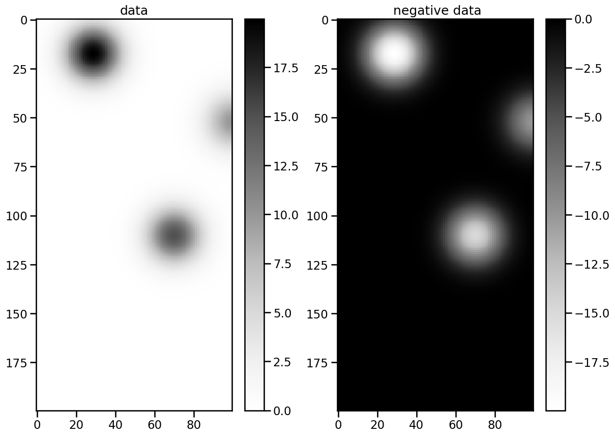
As you can see the data has 3 maxima/minima with different extremal values. To capture these, we use list comprehensions to obtain multiple thresholds in the range of the data:
[5]:
thresholds = [i for i in range(9, 18)]
neg_thresholds = [-i for i in range(9, 18)]
These can now be passed as arguments to feature_detection_multithreshold(). With the target-keyword we can set a flag whether to search for minima or maxima. The standard is "maxima".
[6]:
%%capture

dxy, dt = tobac.utils.get_spacings(data)

features = tobac.feature_detection_multithreshold(
    data, dxy, thresholds, target="maximum"
)
features_inv = tobac.feature_detection_multithreshold(
    neg_data, dxy, neg_thresholds, target="minimum"
)
Let’s scatter the detected features onto frame 50 of the dataset and create colorbars for the threshold values:
[7]:
mask_1 = features["frame"] == n
mask_2 = features_inv["frame"] == n

fig, (ax1, ax2) = plt.subplots(ncols=2, figsize=(14, 10))

ax1.imshow(data.data[50], cmap="Greys")
im1 = ax1.scatter(
    features.where(mask_1)["hdim_2"],
    features.where(mask_1)["hdim_1"],
    c=features.where(mask_1)["threshold_value"],
    cmap="tab10",
)
cbar = plt.colorbar(im1, ax=ax1)
cbar.ax.set_ylabel("threshold")

ax2.imshow(neg_data.data[50], cmap="Greys")
im2 = ax2.scatter(
    features_inv.where(mask_2)["hdim_2"],
    features_inv.where(mask_2)["hdim_1"],
    c=features_inv.where(mask_2)["threshold_value"],
    cmap="tab10",
)
cbar = plt.colorbar(im2, ax=ax2)
cbar.ax.set_ylabel("threshold")
[7]:
Text(0, 0.5, 'threshold')
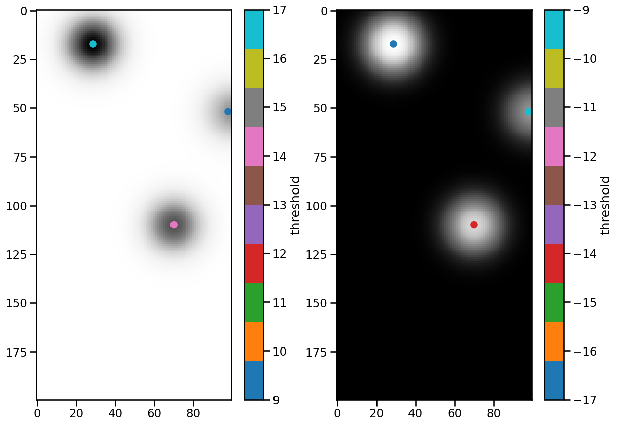
The three features were found in both data sets, and the color bars indicate which threshold they belong to. When using multiple thresholds, note that the order of the list is important. Each feature is assigned the threshold value that was reached last. Therefore, it makes sense to start with the lowest value in case of maxima.
Feature Position
To explore the influence of the position_threshold flag we need a radially asymmetric feature. Let’s create a simple one by adding two 2d-gaussians and add an extra dimension for the time, which is required for working with tobac:
[8]:
x = np.linspace(-2, 2)
y = np.linspace(-2, 2)
xx, yy = np.meshgrid(x, y)

exp1 = 1.5 * np.exp(-((xx + 0.5) ** 2 + (yy + 0.5) ** 2))
exp2 = 0.5 * np.exp(-((0.5 - xx) ** 2 + (0.5 - yy) ** 2))

asymmetric_data = np.expand_dims(exp1 + exp2, axis=0)

plt.figure(figsize=(10, 10))
plt.imshow(asymmetric_data[0])
plt.colorbar(shrink=0.8)
[8]:
<matplotlib.colorbar.Colorbar at 0x1377ed290>
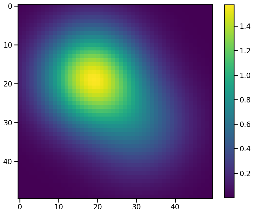
To feed this data into the feature detection we need to convert it into an xarray.DataArray. Before we do that we select an arbitrary time and date for the single frame of our synthetic field:
[9]:
date = np.datetime64(
    "2022-04-01T00:00",
)
assym = xr.DataArray(
    data=asymmetric_data, coords={"time": np.expand_dims(date, axis=0), "y": y, "x": x}
)
assym
[9]:
<xarray.DataArray (time: 1, y: 50, x: 50)> Size: 20kB
array([[[0.01666536, 0.02114886, 0.02648334, ..., 0.00083392,
         0.00058509, 0.00040694],
        [0.02114886, 0.02683866, 0.03360844, ..., 0.00109464,
         0.00077154, 0.0005393 ],
        [0.02648334, 0.03360844, 0.04208603, ..., 0.00142435,
         0.00100896, 0.00070907],
        ...,
        [0.00083392, 0.00109464, 0.00142435, ..., 0.01405279,
         0.01121917, 0.00883872],
        [0.00058509, 0.00077154, 0.00100896, ..., 0.01121917,
         0.00895731, 0.00705704],
        [0.00040694, 0.0005393 , 0.00070907, ..., 0.00883872,
         0.00705704, 0.00556009]]])
Coordinates:
  * time     (time) datetime64[ns] 8B 2022-04-01
  * y        (y) float64 400B -2.0 -1.918 -1.837 -1.755 ... 1.837 1.918 2.0
* x (x) float64 400B -2.0 -1.918 -1.837 -1.755 ... 1.837 1.918 2.0Since we do not have a dt in this dataset, we can not use the get_spacings()-utility this time and need to calculate the dxy spacing manually:
[10]:
dxy = assym.diff("x")
Finally, we choose a threshold in the datarange and apply the feature detection with the four position_threshold flags - ‘center’ - ‘extreme’ - ‘weighted_diff’ - ‘weighted_abs’
[11]:
%%capture

threshold = 0.2
features_center = tobac.feature_detection_multithreshold(
    assym, dxy, threshold, position_threshold="center"
)
features_extreme = tobac.feature_detection_multithreshold(
    assym, dxy, threshold, position_threshold="extreme"
)
features_diff = tobac.feature_detection_multithreshold(
    assym, dxy, threshold, position_threshold="weighted_diff"
)
features_abs = tobac.feature_detection_multithreshold(
    assym, dxy, threshold, position_threshold="weighted_abs"
)
[12]:
plt.figure(figsize=(10, 10))
plt.imshow(assym[0])
plt.scatter(
    features_center["hdim_2"],
    features_center["hdim_1"],
    color="black",
    marker="x",
    label="center",
)
plt.scatter(
    features_extreme["hdim_2"],
    features_extreme["hdim_1"],
    color="red",
    marker="x",
    label="extreme",
)
plt.scatter(
    features_diff["hdim_2"],
    features_diff["hdim_1"],
    color="purple",
    marker="x",
    label="weighted_diff",
)
plt.scatter(
    features_abs["hdim_2"],
    features_abs["hdim_1"],
    color="green",
    marker="+",
    label="weighted_abs",
)
plt.colorbar(shrink=0.8)
plt.legend()
[12]:
<matplotlib.legend.Legend at 0x1377f2b10>
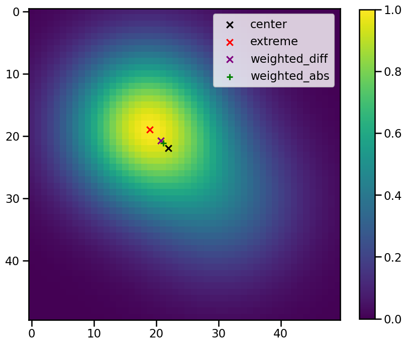
As you can see this parameter specifies how the postion of the feature is defined. These are the descriptions given in the code:
extreme: get position as max/min position inside the identified region
center : get position as geometrical centre of identified region
weighted_diff: get position as centre of identified region, weighted by difference from the threshold
weighted_abs: get position as centre of identified region, weighted by absolute values if the field
Sigma Parameter for Smoothing of Noisy Data
Before the features are searched a gausian filter is applied to the data in order to smooth it. So let’s import the filter used by tobac for a demonstration:
[13]:
from scipy.ndimage import gaussian_filter
This filter works performing a convolution of a (in our case 2-dimensional) gaussian function
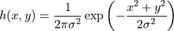
with our data and with this parameter we set the value of  .
.
The effect of this filter can best be demonstrated on very sharp edges in the input. Therefore we create an array from a boolean mask of another 2d-Gaussian, which has only values of 0 or 1:
[14]:
x = np.linspace(-2, 2)
y = np.linspace(-2, 2)
xx, yy = np.meshgrid(x, y)

exp = np.exp(-(xx**2 + yy**2))

gaussian_data = np.expand_dims(exp, axis=0)
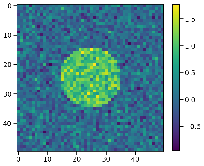
and we add some random noise to it:
[15]:
np.random.seed(54321)

noise = 0.3 * np.random.randn(*gaussian_data.shape)
data_sharp = np.array(gaussian_data > 0.5, dtype="float32")

data_sharp += noise

plt.figure(figsize=(8, 8))
plt.imshow(data_sharp[0])
plt.colorbar(shrink=0.8)
[15]:
<matplotlib.colorbar.Colorbar at 0x137d40250>
If we apply this filter to the data with increasing sigmas, increasingly smoothed data will be the result:
[16]:
non_smooth_data = gaussian_filter(data_sharp, sigma=0)
smooth_data = gaussian_filter(data_sharp, sigma=1)
smoother_data = gaussian_filter(data_sharp, sigma=5)

fig, axes = plt.subplots(ncols=3, figsize=(16, 10))

im0 = axes[0].imshow(non_smooth_data[0], vmin=0, vmax=1)
axes[0].set_title(r"$\sigma = 0$")

im1 = axes[1].imshow(smooth_data[0], vmin=0, vmax=1)
axes[1].set_title(r"$\sigma = 1$")

im2 = axes[2].imshow(smoother_data[0], vmin=0, vmax=1)
axes[2].set_title(r"$\sigma = 5$")

cbar = fig.colorbar(im1, ax=axes.tolist(), shrink=0.4)
cbar.set_ticks(np.linspace(0, 1, 11))
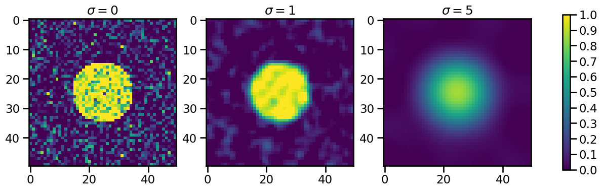
This is what happens in the background, when the feature_detection_multithreshold() function is called. The default value of sigma_threshold is 0.5. The next step is trying to detect features of the dataset with these sigma_threshold values. We first need an xarray DataArray again:
[17]:
date = np.datetime64("2022-04-01T00:00")
input_data = xr.DataArray(
    data=data_sharp, coords={"time": np.expand_dims(date, axis=0), "y": y, "x": x}
)
Now we set a threshold and detect the features:
[18]:
%%capture

threshold = 0.9
features_sharp = tobac.feature_detection_multithreshold(
    input_data, dxy, threshold, sigma_threshold=0
)
features_smooth = tobac.feature_detection_multithreshold(
    input_data, dxy, threshold, sigma_threshold=1
)
features_smoother = tobac.feature_detection_multithreshold(
    input_data, dxy, threshold, sigma_threshold=5
)
Attempting to plot the results
[19]:
fig, axes = plt.subplots(ncols=3, figsize=(14, 10))
plot_kws = dict(
    color="red",
    marker="s",
    s=100,
    edgecolors="w",
    linewidth=3,
)

im0 = axes[0].imshow(input_data[0])
axes[0].set_title(r"$\sigma = 0$")
axes[0].scatter(
    features_sharp["hdim_2"], features_sharp["hdim_1"], label="features", **plot_kws
)
axes[0].legend()

im0 = axes[1].imshow(input_data[0])
axes[1].set_title(r"$\sigma = 1$")
axes[1].scatter(features_smooth["hdim_2"], features_smooth["hdim_1"], **plot_kws)

im0 = axes[2].imshow(input_data[0])
axes[2].set_title(r"$\sigma = 5$")
try:
    axes[2].scatter(
        features_smoother["hdim_2"], features_smoother["hdim_1"], **plot_kws
    )
except:
    print("WARNING: No Feature Detected!")
WARNING: No Feature Detected!
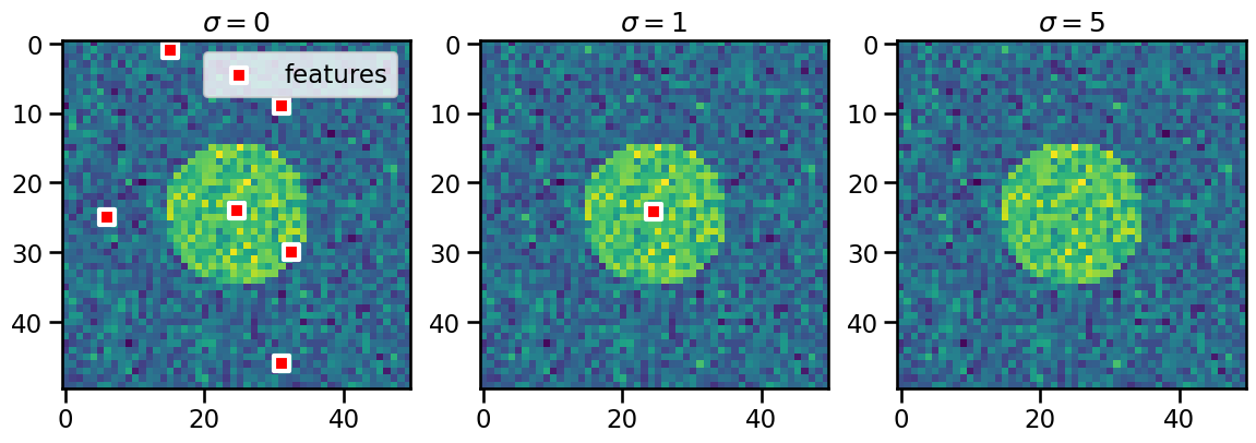
Noise may cause some false detections (left panel) that are significantly reduced when a suitable smoothing parameter is chosen (middle panel).
Band-Pass Filter for Input Fields via Parameter wavelength_filtering
This parameter can be understood best, when looking at real instead of snythethic data. An example of usage is given here