Methods and Parameters for Linking

Linking assigns the detected features and segments in each timestep to trajectories, to enable an analysis of their time evolution. We will cover the topics:

• Understanding the Linking Output

• Defining a Search Radius

• Working with the Subnetwork

• Timescale of the Tracks

• Gappy Tracks

• Other Parameters

We start by loading the usual libraries:

import matplotlib.pyplot as plt
import numpy as np
import xarray as xr

%matplotlib inline

import seaborn as sns

sns.set_context("talk")


import warnings

warnings.filterwarnings("ignore")

import tobac
import tobac.testing

Understanding the Linking Output

Since it has a time dimension, the sample data from the testing utilities is also suitable for a demonstration of this step. The chosen method creates 2-dimensional sample data with up to 3 moving blobs at the same. So, our expectation is to obtain up to 3 tracks.

At first, loading in the data and performing the usual feature detection is required:

%%capture

data = tobac.testing.make_sample_data_2D_3blobs_inv(data_type="xarray")
dxy, dt = tobac.utils.get_spacings(data)
features = tobac.feature_detection_multithreshold(
    data, dxy, threshold=1, position_threshold="weighted_abs"
)

Now the linking via trackpy can be performed. Notice that the temporal spacing is also a required input this time. Additionally, it is necessary to provide either a maximum speed v_max or a maximum search range d_max. Here we use a maximum speed of 100 m/s:

track = tobac.linking_trackpy(features, data, dt=dt, dxy=dxy, v_max=100)

Frame 69: 2 trajectories present.

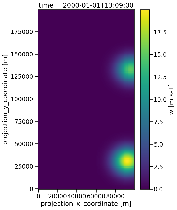
The output tells us, that in the final frame 69 two trajecteries where still present. If we checkout this frame via xarray.plot method, we can see that this corresponds to the two present features there, which are assigned to different trajectories.

plt.figure(figsize=(6, 9))
data.isel(time=69).plot(x="x", y="y")

<matplotlib.collections.QuadMesh at 0x1351a7050>

The track dataset contains two new variables, cell and time_cell. The first assigns the features to one of the found trajectories by an integer and the second specifies how long the feature has been present already in the data.

track[["cell", "time_cell"]][:20]

	cell	time_cell
0	1	0 days 00:00:00
1	1	0 days 00:01:00
2	1	0 days 00:02:00
3	1	0 days 00:03:00
4	1	0 days 00:04:00
5	1	0 days 00:05:00
6	1	0 days 00:06:00
7	1	0 days 00:07:00
8	1	0 days 00:08:00
9	1	0 days 00:09:00
10	1	0 days 00:10:00
11	1	0 days 00:11:00
12	1	0 days 00:12:00
13	1	0 days 00:13:00
14	1	0 days 00:14:00
15	1	0 days 00:15:00
16	1	0 days 00:16:00
17	1	0 days 00:17:00
18	1	0 days 00:18:00
19	1	0 days 00:19:00

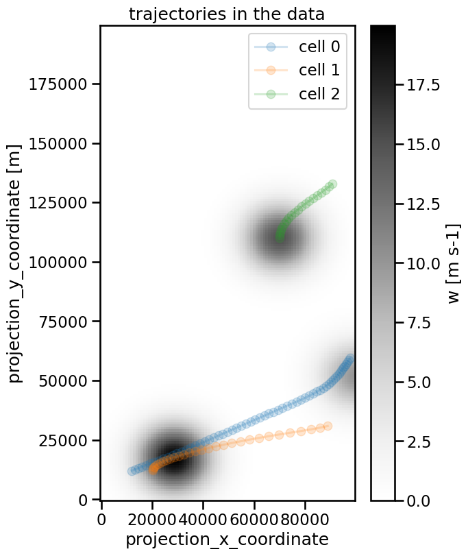
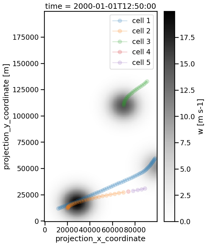
Since we know that this dataset contains 3 features, we can visualize the found tracks with masks created from the cell variable:

fig, ax = plt.subplots(ncols=1, nrows=1, figsize=(6, 9))

data.isel(time=50).plot(ax=ax, x="x", y="y", cmap="Greys")

for i, cell_track in track.groupby("cell"):
    cell_track.plot(
        x="projection_x_coordinate",
        y="projection_y_coordinate",
        ax=ax,
        marker="o",
        alpha=0.2,
        label="cell {0}".format(int(i)),
    )


ax.set_title("trajectories in the data")
plt.legend()

<matplotlib.legend.Legend at 0x1348a2350>

The cells have been specified with different velocities that also change in time. tobac retrieves the following values for our test data:

vel = tobac.analysis.calculate_velocity(track)

fig, ax = plt.subplots(ncols=1, nrows=1, figsize=(12, 6))

for i, vc in vel.groupby("cell"):
    # get velocity as xarray Dataset
    v = vc.to_xarray()["v"]
    v = v.assign_coords({"frame": vc.to_xarray()["frame"]})

    v.plot(x="frame", ax=ax, label="cell {0}".format(int(i)))

    ax.set_ylabel("estimated velocity / (m/s)")

ax.set_title("velocities of the cell tracks")
plt.legend()

<matplotlib.legend.Legend at 0x1351bf250>

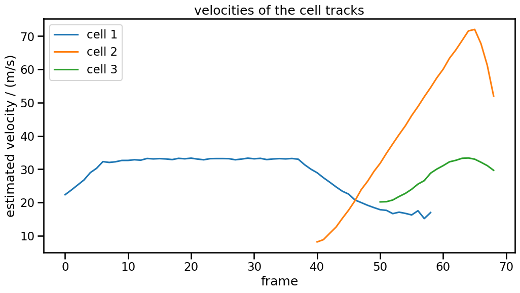
Interpretation:

• “cell 1” is actually specified with constant velocity. The initial increase and the final decrease come from edge effects, i.e. that the blob corresponding to “cell 1” has parts that that go beyond the border.

• “cell 2” and “cell 3” are specified with linearily increasing x-component of the velocity. The initial speed-up is due to the square-root behavior of the velocity magnitude. The final decrease however come again from edge effects.

The starting point of the cell index is of course arbitrary. If we want to change it from 1 to 0 we can do this with the cell_number_start parameter:

track = tobac.linking_trackpy(
    features, data, dt=dt, dxy=dxy, v_max=100, cell_number_start=0
)

fig, ax = plt.subplots(ncols=1, nrows=1, figsize=(6, 9))

data.isel(time=50).plot(ax=ax, x="x", y="y", cmap="Greys")

for i, cell_track in track.groupby("cell"):
    cell_track.plot(
        x="projection_x_coordinate",
        y="projection_y_coordinate",
        ax=ax,
        marker="o",
        alpha=0.2,
        label="cell {0}".format(int(i)),
    )

ax.set_title("trajectories in the data")
plt.legend()

Frame 69: 2 trajectories present.

<matplotlib.legend.Legend at 0x13598a350>

The linking in tobac is performed with methods of the trackpy-library. Currently, there are two methods implemented, ‘random’ and ‘predict’. These can be selected with the method keyword. The default is ‘random’.

track_p = tobac.linking_trackpy(
    features, data, dt=dt, dxy=dxy, v_max=100, method_linking="predict"
)

Frame 69: 2 trajectories present.

Defining a Search Radius

If you paid attention to the input of the linking_trackpy() function you noticed that we used the parameter v_max there. The reason for this is that it would take a lot of computation time to check the whole data of a frame for the next position of a feature from the previous frame with the Crocker-Grier linking algorithm. Therefore the search is restricted to a circle around a position predicted by different methods implemented in trackpy.

The speed we defined before specifies such a radius timestep via

By reducing the maximum speed from 100 m/s to 70 m/s we will find more cell tracks, because a feature that is not assigned to an existing track will be used as a starting point for a new one:

track = tobac.linking_trackpy(features, data, dt=dt, dxy=dxy, v_max=70)

fig, ax = plt.subplots(ncols=1, nrows=1, figsize=(6, 9))

data.isel(time=50).plot(ax=ax, x="x", y="y", cmap="Greys")

for i, cell_track in track.groupby("cell"):
    cell_track.plot(
        x="projection_x_coordinate",
        y="projection_y_coordinate",
        ax=ax,
        marker="o",
        alpha=0.2,
        label="cell {0}".format(int(i)),
    )

plt.legend()

Frame 69: 2 trajectories present.

<matplotlib.legend.Legend at 0x13598a290>

Above you see that previously orange track is split into three parts because the considered cell moves so fast.

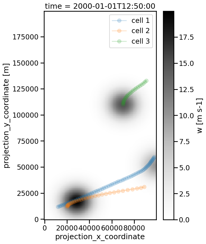
The same effect can be achieved by directly reducing the maximum search range with the d_max parameter to

because

for m/s in our case.

track = tobac.linking_trackpy(features, data, dt=dt, dxy=dxy, d_max=4200)

fig, ax = plt.subplots(ncols=1, nrows=1, figsize=(6, 9))

data.isel(time=50).plot(ax=ax, x="x", y="y", cmap="Greys")

for i, cell_track in track.groupby("cell"):
    cell_track.plot(
        x="projection_x_coordinate",
        y="projection_y_coordinate",
        ax=ax,
        marker="o",
        alpha=0.2,
        label="cell {0}".format(int(i)),
    )

plt.legend()

Frame 69: 2 trajectories present.

<matplotlib.legend.Legend at 0x1365638d0>

v_max and d_max should not be used together, because they both specify the same qunatity, namely the search range, but it is neccery to set at least one of these parameters.

Working with the Subnetwork

If we increase v_max or d_max it can happen that more than one feature of the previous timestep is in the search range. The selection of the best matching feature from the set of possible features (which is called the subnetwork, for a more in depth explanation have a look here) is the most time consuming part of the linking process. For this reason, it is possible to limit the number of features in the search range via the subnetwork_size parameter. The tracking will result in a trackpy.SubnetOversizeException if more features than specified there are in the search range. We can simulate this situation by setting a really high value for v_max and 1 for the subnetwork_size:

from trackpy import SubnetOversizeException

try:
    track = tobac.linking_trackpy(
        features, data, dt=dt, dxy=dxy, v_max=1000, subnetwork_size=1
    )
    print("tracking successful")

except SubnetOversizeException as e:
    print("Tracking not possible because the {}".format(e))

Frame 57: 3 trajectories present.
Tracking not possible because the Subnetwork contains 2 points

The default value for this parameter is 30 and can be accessed via:

import trackpy as tp

tp.linking.Linker.MAX_SUB_NET_SIZE

1

It is important to highlight that if the linking_trackpy()-function is called with a subnetwork_size different from 30, this number will be the new default. This is the reason, why the value is 1 at this point.

Adaptive Search

A way of dealing with SubnetOversizeExceptions is adaptive search. An extensive description can be found here.

If the subnetwork is too large, the search range is reduced iteratively by multiplying it with the adaptive_step. The adaptive_stop-parameter is the lower limit of the search range. If it is reached and the subnetwork is still too large, a SubnetOversizeException is thrown. Notice that as soon as adaptive search is used, a different limit of the subnetwork size applies, which needs to be specified by hand at the moment:

tp.linking.Linker.MAX_SUB_NET_SIZE_ADAPTIVE = 1

Now the tracking can be performed and will no longer result in an exception:

try:
    track = tobac.linking_trackpy(
        features, data, dt=dt, dxy=dxy, v_max=1000, adaptive_stop=10, adaptive_step=0.9
    )
    print("tracking successful!")

    fig, ax = plt.subplots(ncols=1, nrows=1, figsize=(6, 9))

    data.isel(time=50).plot(ax=ax, x="x", y="y", cmap="Greys")

    for i, cell_track in track.groupby("cell"):
        cell_track.plot(
            x="projection_x_coordinate",
            y="projection_y_coordinate",
            ax=ax,
            marker="o",
            alpha=0.2,
            label="cell {0}".format(int(i)),
        )

    plt.legend()

except SubnetOversizeException as e:
    print("Tracking not possible because the {}".format(e))

Frame 69: 2 trajectories present.
tracking successful!

If adaptive_stop is specified, adaptive_step needs to be specified as well.

Timescale of the Tracks

If we want to limit our analysis to long living features of the dataset it is possible to exclude tracks which only cover few timesteps. This is done by setting a lower bound for those via the stups parameter. In our test data, only the first cell exceeds 50 time steps:

track = tobac.linking_trackpy(features, data, dt=dt, dxy=dxy, v_max=100, stubs=50)

Frame 69: 2 trajectories present.

Now, the DataFrame track contains two types (two categories) of cells: 1. tracked cells: connected with cell tracks 2. untracked cells: not connected

The first type (“tracked cells”) is what you know and what you have already worked with. But the 2nd type (“untracked cells”) is new. All untracked cells are marked with the cell index -1 and thus collected in a buffer space.

tracked_cells_only = track.where(track.cell > 0)
untracked_cells = track.where(track.cell == -1)

Now, the track dataset is split into two parts. Let’s have a look:

fig, ax = plt.subplots(ncols=1, nrows=1, figsize=(6, 9))

data.isel(time=50).plot(ax=ax, x="x", y="y", cmap="Greys")

for i, cell_track in tracked_cells_only.groupby("cell"):
    cell_track.plot(
        x="projection_x_coordinate",
        y="projection_y_coordinate",
        ax=ax,
        marker="o",
        alpha=0.2,
        label="cell {0}".format(int(i)),
    )

for i, cell_track in untracked_cells.groupby("cell"):
    cell_track.plot(
        x="projection_x_coordinate",
        y="projection_y_coordinate",
        ax=ax,
        color="gray",
        marker="*",
        label="untracked cells",
        lw=0,
        alpha=0.2,
    )

plt.legend()

<matplotlib.legend.Legend at 0x137046190>

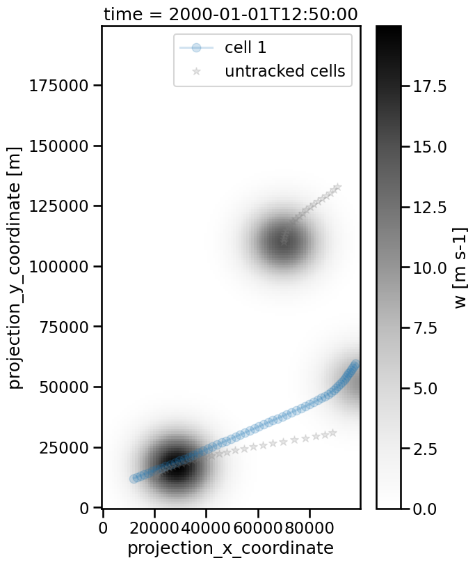
Analogius to the search range, there is a second option for that called time_cell_min. This defines a minimum of time in seconds for a cell to appear as tracked:

track = tobac.linking_trackpy(
    features,
    data,
    dt=dt,
    dxy=dxy,
    v_max=100,
    time_cell_min=60 * 50,  # means 50 steps of 60 seconds
)

tracked_cells_only = track.where(track.cell > 0)

untracked_cells = track.where(track.cell == -1)

Frame 69: 2 trajectories present.

fig, ax = plt.subplots(ncols=1, nrows=1, figsize=(6, 9))

data.isel(time=50).plot(ax=ax, x="x", y="y", cmap="Greys")

for i, cell_track in tracked_cells_only.groupby("cell"):
    cell_track.plot(
        x="projection_x_coordinate",
        y="projection_y_coordinate",
        ax=ax,
        marker="o",
        alpha=0.2,
        label="cell {0}".format(int(i)),
    )

for i, cell_track in untracked_cells.groupby("cell"):
    cell_track.plot(
        x="projection_x_coordinate",
        y="projection_y_coordinate",
        ax=ax,
        color="gray",
        marker="*",
        label="untracked cells",
        lw=0,
        alpha=0.2,
    )

plt.legend()

<matplotlib.legend.Legend at 0x133e9f550>

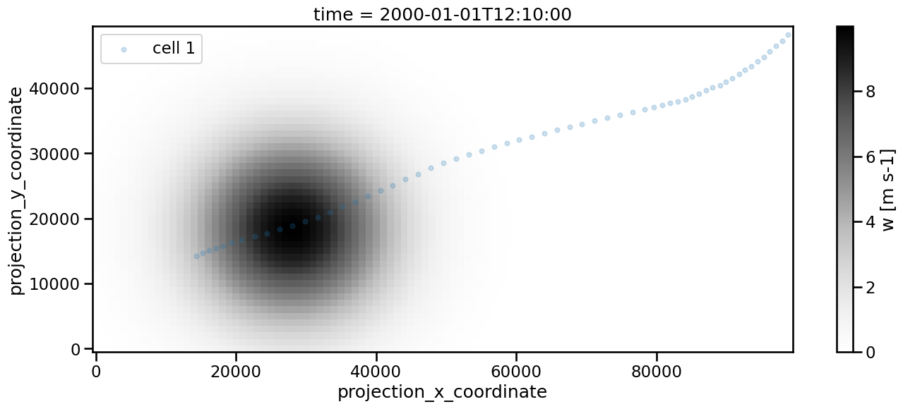
Gappy Tracks

If the data is noisy, an object may disappear for a few frames and then reappear. Such features can still be linked by setting the memory parameter with an integer. This defines the number of timeframes a feature can vanish and still get tracked as one cell. We demonstrate this on a simple dataset with only one feature:

data = tobac.testing.make_simple_sample_data_2D(data_type="xarray")
dxy, dt = tobac.utils.get_spacings(data)
features = tobac.feature_detection_multithreshold(data, dxy, threshold=1)
track = tobac.linking_trackpy(features, data, dt=dt, dxy=dxy, v_max=1000)

fig, ax = plt.subplots(ncols=1, nrows=1, figsize=(16, 6))

data.isel(time=10).plot(ax=ax, x="x", y="y", cmap="Greys")

for i, cell_track in track.groupby("cell"):
    cell_track.plot.scatter(
        x="projection_x_coordinate",
        y="projection_y_coordinate",
        ax=ax,
        marker="o",
        alpha=0.2,
        label="cell {0}".format(int(i)),
    )

plt.legend()

Frame 59: 1 trajectories present.

<matplotlib.legend.Legend at 0x136b09c10>

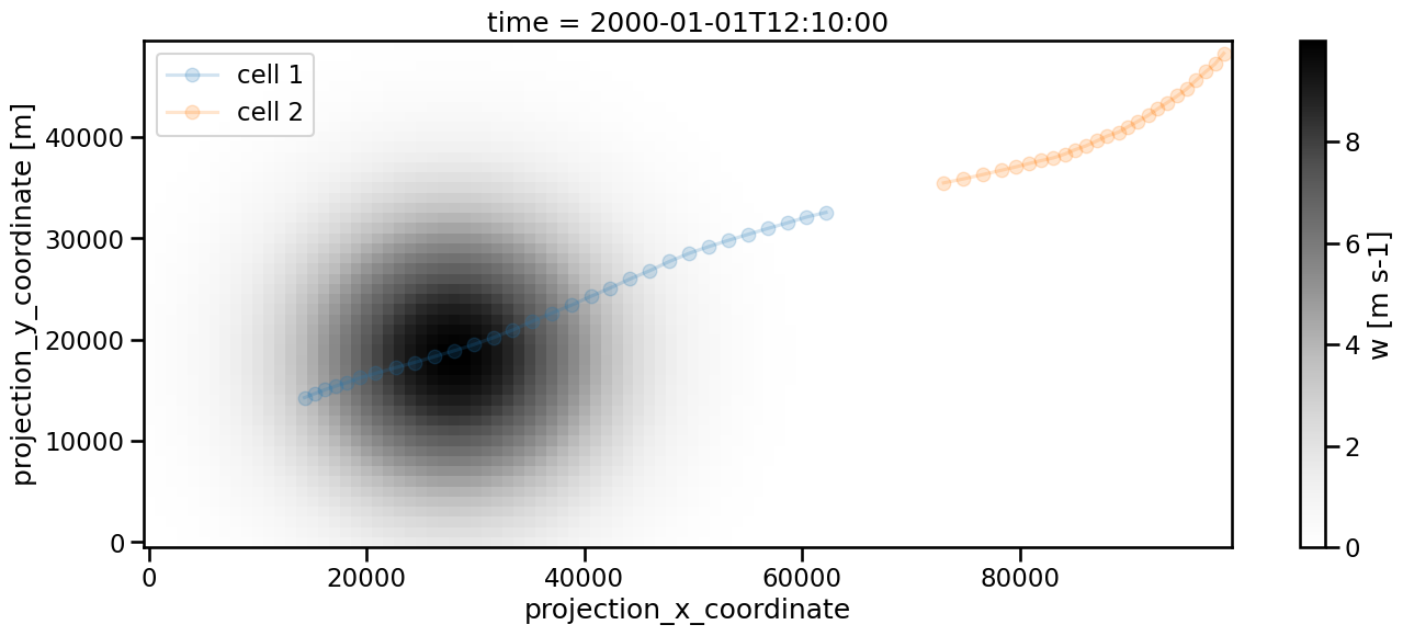
To simulate a gap in the data we set 5 timeframes to 0:

data[30:35] = data[30] * 0

If we apply feature detection and linking to this modified dataset, we will now get two cells:

features = tobac.feature_detection_multithreshold(data, dxy, threshold=1)
track = tobac.linking_trackpy(features, data, dt=dt, dxy=dxy, v_max=1000)

fig, ax = plt.subplots(ncols=1, nrows=1, figsize=(16, 6))

data.isel(time=10).plot(ax=ax, x="x", y="y", cmap="Greys")

for i, cell_track in track.groupby("cell"):
    cell_track.plot(
        x="projection_x_coordinate",
        y="projection_y_coordinate",
        ax=ax,
        marker="o",
        alpha=0.2,
        label="cell {0}".format(int(i)),
    )

plt.legend()

Frame 59: 1 trajectories present.

<matplotlib.legend.Legend at 0x136a5fe90>

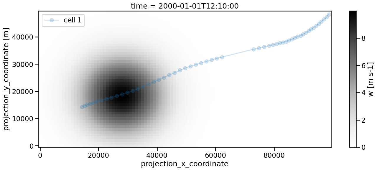
We can avoid that by setting memory to a sufficiently high number. 5 is of course sufficient in our case as the situation is artificially created, but with real data this would require some fine tuning. Keep in mind that the search radius needs to be large enough to reach the next feature position. This is the reason for setting v_max to 1000 in the linking process.

features = tobac.feature_detection_multithreshold(data, dxy, threshold=1)
track = tobac.linking_trackpy(features, data, dt=dt, dxy=dxy, v_max=1000, memory=5)

fig, ax = plt.subplots(ncols=1, nrows=1, figsize=(16, 6))

data.isel(time=10).plot(ax=ax, cmap="Greys")

for i, cell_track in track.groupby("cell"):
    cell_track.plot(
        x="projection_x_coordinate",
        y="projection_y_coordinate",
        ax=ax,
        marker="o",
        alpha=0.2,
        label="cell {0}".format(int(i)),
    )

plt.legend()

Frame 59: 1 trajectories present.

<matplotlib.legend.Legend at 0x136bd2c10>

vel = tobac.analysis.calculate_velocity(track)

fig, ax = plt.subplots(ncols=1, nrows=1, figsize=(12, 6))

for i, vc in vel.groupby("cell"):
    # get velocity as xarray Dataset
    v = vc.to_xarray()["v"]
    v = v.assign_coords({"frame": vc.to_xarray()["frame"]})
    v.plot(x="frame", ax=ax, label="cell {0}".format(int(i)), marker="x")

    ax.set_ylabel("estimated velocity / (m/s)")

ax.axvspan(30, 35, color="gold", alpha=0.3)
ax.set_title("velocities of the cell tracks")
plt.legend()

<matplotlib.legend.Legend at 0x136dce390>

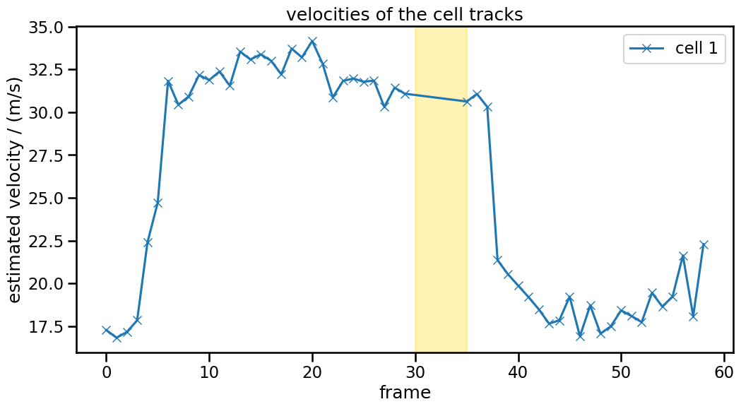
Velocity calculations work well across the gap (marked with yellow above). The initial and final drop in speed comes again from edge effects.

Other Parameters

The parameters d_min_, extrapolate and order do not have a working implmentation in tobac V2 at the moment.